

Follow-up to Post 2: “How to Actually Upgrade to AAD”
The first post argued that FRTB is a compute problem, not a modelling problem. The second showed that migrating to AAD doesn’t require rewriting your library. Both posts assumed you have an existing codebase.
Several people asked the obvious next question: what if we’re starting fresh? New desk, new risk engine, greenfield build. What should the architecture look like if you design around differentiation from day one?
This is what we built. The patterns are general.
One principle
Separate the what from the how.
Business logic is written in readable code. Python or C++, whichever your quants prefer. This code runs once. It defines the computation. The AD compiler records it into a kernel.
The kernel is what runs in production. It replays millions of times with SIMD vectorization and computes adjoint Greeks in a single backward pass.
Your quant code can afford to be clear instead of clever. It executes once during recording. The millions of Monte Carlo paths, the sensitivities, the stress scenarios all run through compiled machine code generated from that single recording.
The type is the architecture
In C++, you write with an active double type. Not double. Not a template that switches between them. Your code uses the active type throughout, and operator overloading captures the computation graph at runtime. No source transformation, no compiler plugins.
In Python, the AD system handles this transparently inside a recording context. You write normal arithmetic. The recording captures it.
Both produce the same compiled kernel. The language choice is about who writes the business logic and how fast they iterate, not about what runs in production.
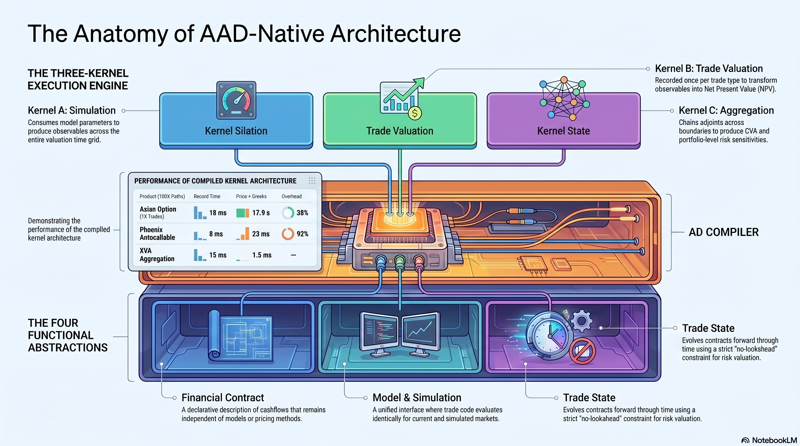
Four abstractions
The architecture has four core components. Each is small enough to implement in a few hundred lines.
Market Observables are just data: spot prices, yield curves, vol surfaces, credit spreads. Snapped independently of any pricing logic. This mirrors how desks already work. Nothing controversial here.
Financial Contract is a declarative description of cashflows. An FX forward is: “At T, party A pays X in EUR, party B pays Y in USD.” No model, no pricing method. The same contract object works for front office, middle office, and risk.
Model and Simulation. The simulation engine exposes a SimulatedMarket interface that looks identical to the market object. Trade code does not change between “evaluate at today’s market” and “evaluate on a simulated path two years from now.” A single kernel can serve both pricing and XVA without modification because of this.
Trade State evolves a contract forward through time. At each step it consumes observables, updates internal state (accrued interest, exercise flags, barrier levels), and emits cashflows. It cannot look ahead. That constraint is what makes the same time-stepping loop work for both valuation and risk.
There is a fifth abstraction, a Decision Layer for optimal control and exercise, but it deserves its own post. That’s Post 4.
Three kernels
Most risk systems run one monolithic computation per portfolio. We split it into three kernels with a clean interface between them.
Kernel A, simulation. Takes model parameters, produces observables at each valuation time. Recorded once per model. Does not know how many trades exist.
Kernel B, trade valuation. Takes observables, produces NPV. Recorded once per trade type. A portfolio of 10,000 swaps with five types means five kernel recordings. Adding another swap of an existing type costs zero recordings. Changing the valuation date costs zero re-recordings. The observables are the interface, and the kernel doesn’t care where they came from.
Kernel C, portfolio aggregation and XVA. Takes portfolio value at each pricing time, produces CVA, DVA, FVA, exposure profiles. Recorded once per netting set. Does not know what instruments are in the portfolio.
The boundary between these kernels is the observable set. Trades consume observables, not curves. Recording is instead of .
Market data changes and new valuation dates require zero re-recordings. Only the simulation kernel depends on the time grid.
Full portfolio risk to model parameters chains across the boundary:
dCVA/dModelParam = dCVA/dV_portfolio × Σ (dNPV/dObservable × dObservable/dModelParam)
Each factor comes from a different kernel’s adjoint. One forward pass and one backward pass per kernel gives you all sensitivities.
What falls out of this
Once you have the three-kernel architecture, pricing and Greeks are just forward plus adjoint. XVA is the three kernels composing. FRTB SA is one adjoint pass producing delta, vega, and curvature by risk class. SIMM is the same adjoint sensitivities fed into ISDA buckets. Calibration is gradient descent on model parameters, same kernel. Stress testing replays with stressed inputs, no re-recording.
These are all the same thing with different inputs. One architecture instead of six systems.
The numbers
We built this and ran it across products of varying complexity. All numbers are from a single machine, 8 threads, compiled kernel evaluation.
| Product | Setup | Record | Price | Price + Greeks | Overhead |
|---|---|---|---|---|---|
| Asian option (1K trades, 100K paths, 252 steps) | MC | 18 ms | 13 s | 17.9 s | 38% |
| Phoenix autocallable (2 assets, 100K paths) | MC | 8 ms | 12 ms | 23 ms | 92% |
| Convertible bond (equity + credit) | Lattice | — | — | — | 4% |
| XVA aggregation (1K scenarios) | Simulation | 15 ms | — | 1.5 ms | — |
Under bump and revalue, each additional risk factor costs another full repricing. Twenty tenor-bucketed rate sensitivities plus spot plus a vol surface is easily 50 to 100 repricings. The adjoint cost is fixed regardless of how many sensitivities you need.
Deployment
The compiled kernel is a pure function. Inputs in, outputs out. No database, no global state, no framework dependency at runtime.
On-premises: a kernel server with in-memory caching, record once, serve many clients over TCP. Cloud: stateless by construction, kernels serialise to disk, load on cold start, fit Lambda or any serverless platform. Embedded: C++ library or Python package, no server, just import and call.
Same core computation, three transport layers.
The tradeoff
Designing around adjoint differentiation means every computation must flow through types that the AD compiler can record. You can’t call into opaque C libraries that use raw double internally and expect Greeks to appear on the other side. Every function in the pricing path needs to speak the active type.
For a greenfield build, this is free. You’re writing it for the first time. For a migration, Post 2 covered the path: one pricer at a time, cohort mirror validation at each step.
The payoff is that differentiation becomes a property of the architecture, not a feature you maintain separately. Greeks, calibration, and regulatory sensitivities all come from the same mechanism. Add a new product and it’s automatically differentiable. A regulator asks for a new sensitivity and it’s already computed.
This is how we built it. The patterns are general.
Next: Post 4 covers what happens when you put neural networks on the same tape as your simulation.
Implemented using AADC, a commercial adjoint AD compiler (matlogica.com). The architecture patterns described here are tool-agnostic — any tape-based AD system that supports control flow recording and kernel compilation could serve the same role.