

Every actuary I’ve talked to about applying adjoint algorithmic differentiation to Variable Annuities has said some version of the same thing: “You can’t do that.”
The ratchet resets are discontinuous. The lapse function is a step function of moneyness. The withdrawal logic is a cascade of if-then-else branches. A 35-year monthly simulation with eight state variables will produce either zero gradients or numerical garbage. And the tape will be enormous.
These objections are correct for naive AD implementations. We solved all of them.
The problem nobody talks about
The computational burden on VA portfolios is growing faster than hardware can keep up.
VM-21 with the new GOES scenarios requires 10,000 full paths, up from the subsets of 1,000 that many companies previously used. LDTI requires quarterly fair-value MRB calculations where changes flow directly through net income. Solvency II’s revision tightens capital requirements and demands nested stochastic simulation: 1,000–5,000 outer scenarios, each requiring 1,000–10,000 inner scenarios for a full liability revaluation.
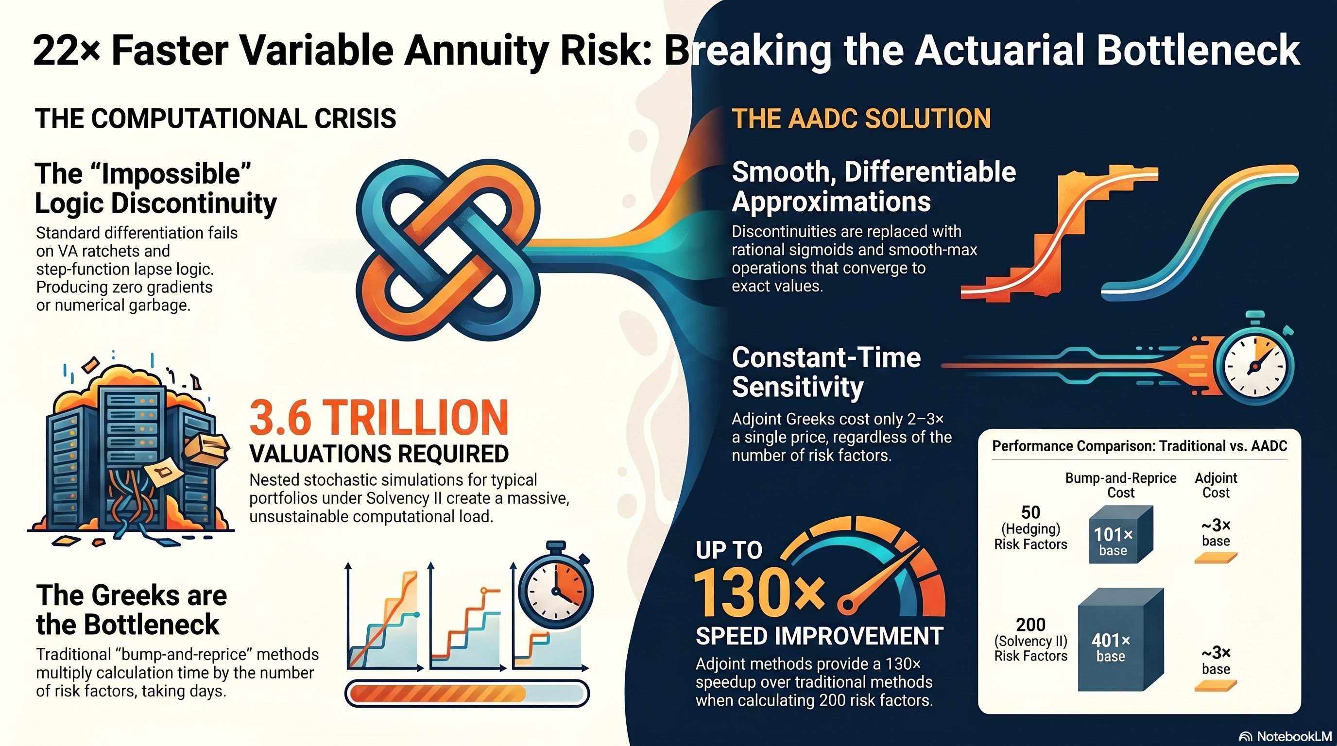
For a typical VA portfolio (100,000 policies, 10,000 outer scenarios, 1,000 inner scenarios, 360 monthly time steps) the full nested calculation is 3.6 trillion valuations. Adding bump-and-reprice Greeks for 100 risk factors multiplies this by 201. Academic estimates put that at over six days on fast hardware.
So companies don’t do it properly. They run fewer scenarios, approximate Greeks with proxy models, and report results with caveats.
The bottleneck is not the price. It’s the Greeks. Hedge ratios, risk factor sensitivities, regulatory stress tests all require bumping one input and repricing the entire portfolio. For 50 risk factors, that’s 101 full evaluations (central differences). For 200 risk factors under a full Solvency II internal model, it’s 401.
How we made it work
The core insight is that every discontinuity in VA contract logic (ratchet resets, lapse staircases, withdrawal splits) can be replaced by a smooth, infinitely differentiable approximation. The approximation converges to the exact function as a sharpness parameter increases. The bias is quantifiable and controllable.
The ratchet reset, , becomes a smooth max. The ITM-dependent lapse staircase becomes a sum of rational sigmoids. The three-way GMWB withdrawal split becomes a composition of smooth min and max operations. Every branch and kink gets the same treatment.
We use rational sigmoids rather than exponential ones. No overflow, cheaper on tape, continuously differentiable. The bias at production sharpness is sub-basis-point on prices after Monte Carlo integration.
One subtlety that catches even experienced practitioners: never use smooth max for accumulating Boolean flags. returns approximately 0.022, not zero. After 420 monthly steps, that bias accumulates to 1.0 — your “never triggered” flag reads as “always triggered.” We use multiplicative Boolean algebra instead. That single fix reduced barrier option errors from 529% to 8%.
What we actually built
Five VA riders, each fully differentiable:
| Product | State Variables | Key Challenge |
|---|---|---|
| GMDB | 4 | Ratchet/rollup anniversary resets |
| GMAB | 3 | European put on account value at maturity |
| GMWB | 5 | Three-way withdrawal split |
| GMWB + Ratchet + Rollup + GMDB | 8 | All combined — ~70% of new VA sales |
| GMIB | 7 | Two-phase: accumulation then annuitisation |
The kernel records the entire multi-decade simulation in a single pass, compiles it to native machine code with AVX vectorisation, and caches the compiled kernel. Market data changes don’t trigger re-recording. Only structural changes do.
The numbers
Greeks via adjoint cost roughly 2–3× a single forward price, regardless of how many risk factors you differentiate against:
| Risk factors | Bump-and-reprice | Adjoint | Speedup |
|---|---|---|---|
| 50 (realistic hedging) | 101× base | ~3× base | 34× |
| 200 (full Solvency II) | 401× base | ~3× base | 130× |
For a VM-21 batch (10,000 policies, 1,000 scenarios, 20 tenor-bucketed Greeks), traditional bump-and-reprice takes an estimated 144 hours. The adjoint kernel does it overnight.
The recording cost is a one-time 1–2 seconds for the most complex products. Amortised across millions of evaluations, it’s noise.
Validation
We validate through three independent checks:
First, a cohort mirror. The same code path runs with plain doubles and with active doubles. Prices must match to machine epsilon. They do, $0.00 difference across all five riders.
Second, adjoint versus finite difference. Adjoint Greeks are compared against central finite differences computed on an entirely separate code path. Relative errors below 1% for Delta, Vega, and Rho across all products.
Third, smooth convergence. As sharpness increases, prices converge monotonically toward the hard-branching reference. The gap shrinks as , confirming the approximation is well-behaved.
131 tests pass across all five riders.
What this unlocks beyond speed
The smooth formulation makes policyholder behaviour assumptions differentiable. We parameterise lapse rates, utilisation rates, and ITM boundaries as ten scalar inputs on the tape. A single adjoint pass produces alongside the market Greeks.
This enables gradient-based calibration, fitting assumptions to observed experience data in ~200 iterations instead of thousands with derivative-free methods. It also enables gradient ascent for worst-case search, finding the policyholder behaviour that maximises insurer cost and directly addressing the regulatory requirement to consider adverse assumptions.
Instead of testing a discrete grid of scenarios, you navigate the full assumption space with exact gradients.
The regulatory reality
VM-21 GOES is effective January 2026 with 10,000 scenarios. LDTI requires quarterly stochastic fair-value calculations. The Solvency II review introduces tougher spread-risk stress tests and increased scrutiny on proxy model accuracy. IFRS 17 demands sensitivity analysis across both market and insurance risks.
Every one of these adds computational load. The industry response has been to buy more hardware, simplify models, or accept approximations. That approach has a ceiling.
The alternative is to compute exact sensitivities to all inputs in one backward pass, at a cost independent of how many risk factors you have. The mathematics has been standard for decades. It trains every neural network in existence. The engineering to make it work for Variable Annuities through 480 months of discontinuous contract logic is what took the effort.
The code does not lie. Five riders, 131 tests, machine-epsilon cohort agreement, sub-percent Greek accuracy. Every branch smooth, every gradient exact.
Implemented using AADC, a commercial adjoint AD compiler (matlogica.com). Originally published on LinkedIn.